[Excel] How to add zero before a number in Excel

Use Apostrophe

The easiest way to add zeros in front of numbers in Excel is to add apostrophe (‘) before zeros.

This automatically converts numbers into texts so you will see a green triangle at the top-left corner of the cell indicating an error. Click “Ignore error” to proceed.

Text Formatting

You can simply change the number format to text to keep the leading zeros in numbers. To do this, follow the instructions below:

1. Right-click on the cell(s) where you want to add the leading zeros.

2. Select Format cells.

                          

3. The Format Cells dialog box will appear. Select Text from the category options.

4. Click OK.

                          

Custom Formatting

If you don't want the data to appear as text and you want to keep the number value, you may apply custom formatting. To do this, follow the instructions below:

1. Right-click on the cell(s) where you want to add the leading zeros.

2. Select Format cells.

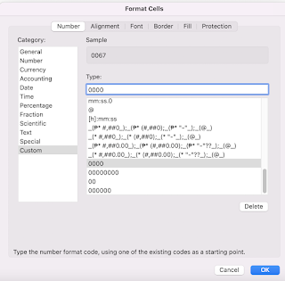
3. The Format Cells dialog box will appear. Select Custom from the category options.

4. Enter zeros in the "Type" box. In the "Sample" box above, it will show how the value will appear in the cell.

5. Click OK.

                                

Apply Formula

TEXT Function

Example:

Where:

B2 = cell number where to get the original value

0000 = string length or the number of digits of the new value

REPT Function

Example:

Where:

0 = value (zero) to be added

2 = number of values (zeros) to be added

B2 = cell number where to get the original value

                

CONCAT Function

Example:

Where:

0000 = number of values (zeros) to be added

B2 = cell number where to get the original value

Use Ampersand

Example:

                                    

Where:

000 = number of values (zeros) to be added

B2 = cell number where to get the original value